Agent Based Simulation for Traffic Analysis

Simulating the traffic of big cities is a big challenge for several reasons, ranging from the difficulties of mathematically formulating the complexity of cars movements at specific times and in everyday situations, to such as an accident or a pothole. At the same time one thing can be taken as a fact: the problem of mobility in large urban centers is costly and directly linked to quality of life.
In megalopolises such as New York, equally complex traffic solutions have been developed and implemented, with synchronized traffic lights trying to minimize congestion. However, these solutions are not easily replicable to other scenarios, especially when the length of the analyzed area becomes too large.
It is (as an example) in this complexity scenario that agent-based simulation is useful. It is not simple to analyze the complex movement of a set of cars throughout the day, but it is (simpler) to imagine the pattern of behavior of a single individual. For example, it is no exaggeration to confidently infer that a person usually leaves for work at 8:30 am and returns home at 6 pm, with an average 30-minute variation. Simple assumptions, when simulated on a large scale, are capable of generating a complex pattern of behavior that would not be easily possible by other techniques.
Agent based simulation
But what is agent-based simulation? Agent-based simulation is nothing more than individual agent simulation (individuals, for example), from the lowest level of interpretation of a phenomenon, used to the develop the understanding of something more complex, arising from the set of individual actions.
For example, the movement of birds flying together is mathematically (and biologically) quite complex. Behind the complexity of these movements, however, lies a pattern of pure simplicity.
 https://www.slideshare.net/premsankarchakkingal/introduction-to-agent-based-modeling-using-netlogo
If we simulate a simple bird flying we can with just a few parameters, understand the result of the set of interactions. In this code available from NetLogo (established ABM analysis software), 3 simple main parameters are used to analyze this case: alignment, separation and cohesion.
GAMA Platform
Although softwares such as NetLogo are most famous for working with agent-based simulation, it is important to understand that each application will require some specificities that may favor either software. The article Agent Based Modeling and Simulation tools: A review of the state-of-the-art software compares the available software. Here we will use the GAMA Platform, due to its good integration with georeferenced data.
The GAMA platform is a simulation software used to simultaneously reproduce n-agents and view them in a graphically updated manner in real time. The platform differential, which has its own language (GAML), is the simple integration with GIS spatial information files. Other software options can be used for the same purpose.
Importing the road files for analysis
To represent the streets that will be used in this analysis, we need them to be in compatible format with shapefile files. Thus, we will use the Transport_v2017.zip file, available at this link.
Once with the files, we should extract the zip file and with some GIS file viewer software of preference, edit what we need. Here we will use the open source QGIS software.
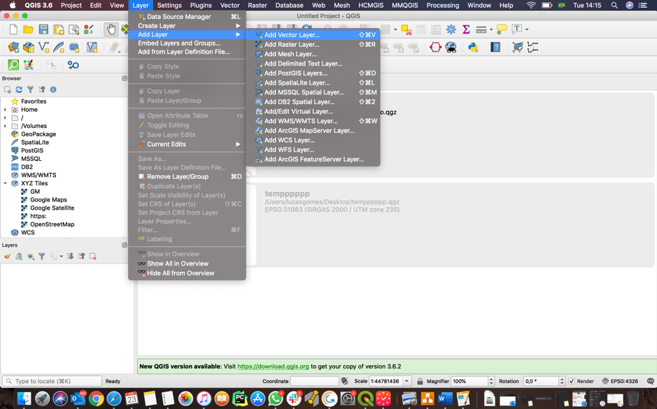
On the QGIS main screen, click Add Vector Layer.
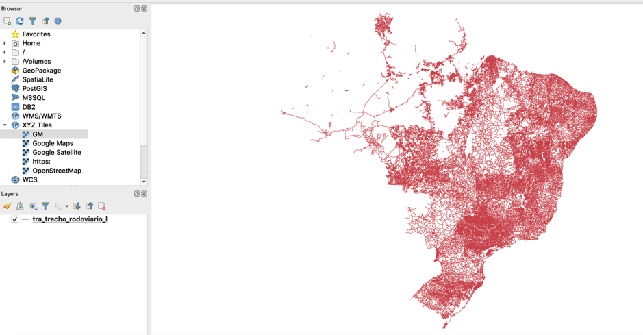
Then choose the file “tra_trecho_rodoviario_I.shp”. After uploading the file, we should have a view of the highways throughout Brazil.
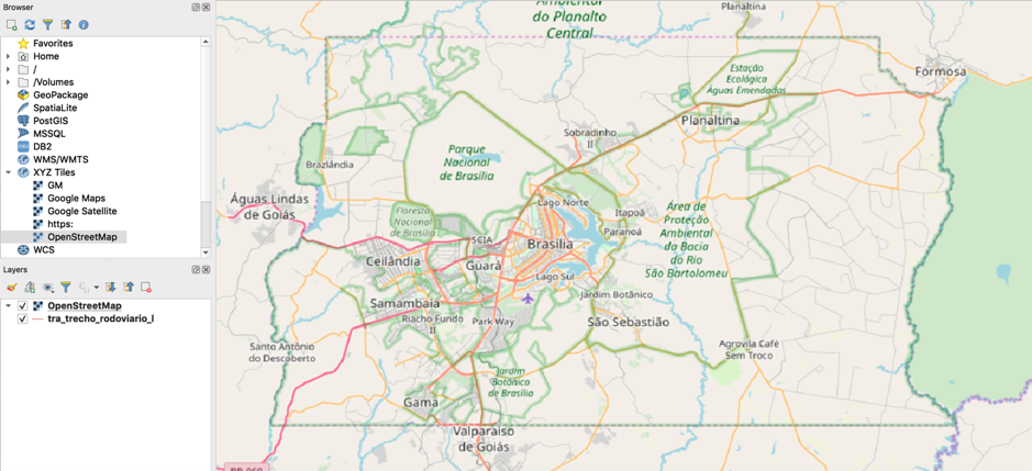
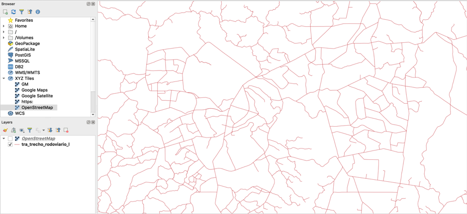
We can then refine our data to have just the desired area, then reduce our analysis space and make the simulation feasible and interpretable. Using the OpenLayers plugin, you can have a cartographic view to assist in the process of choosing the desired region. With this layer activated on the lower left side, we can zoom in on the Federal District region, then deselect the map layer and view only the highways there.
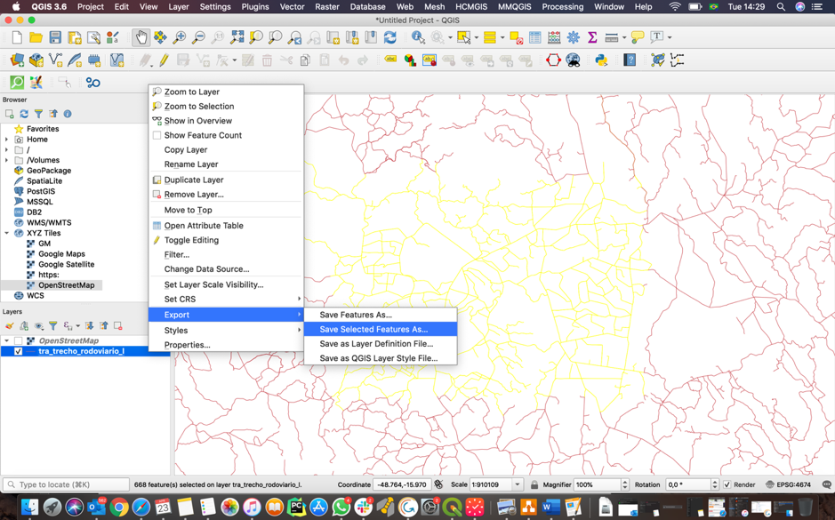
With the layer selected on the lower left side, we can use the select feature by area tool (yellow button) and choose the desired region by dragging the mouse over the desired area.
With the selected area highlighted, we can right-click on the tra_trecho_rodoviario_I layer and choose save selected features as, and choose to save the file in shapefile (.shp) format.
Okay, now we have the base files for the highways that we will use in our simulation.
GAMA Language – GAML
Agent-based simulation are quite similar to object-oriented programming. We have global variables and properties, as well as agents, which are defined with general and specific properties. Thus we can inherit values and functions at different levels to form the agent with the characteristics we need.
The simulation works on ticks, which act as passages of time. When starting a simulation in GAMA, only the initial tick is executed, and all others are then executed accordingly to the simulated time passage or specific criteria, which need to be predetermined.
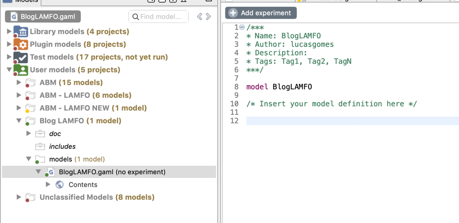
To start our simulation, we must first create a project and a .gaml file.

Initially two main directories are created, includes (where will all files that will serve as input to our model be) and models (where our code will be).
With the files generated in the previous step, we must place them in the includes folder, and import them into the Global definition with the following command:
global{
	file shape_file_roads <- ("../includes/rodoviasdf.shp");
	}
We take the opportunity to define the geometry of the streets.
global{
	file shape_file_roads <- ("../includes/rodoviasdf.shp");
	geometry shape <- envelope(shape_file_roads);
	}
Next we need to define what the highway agent will be like. Here, let’s just say that the street will look like the geometry that the file itself brings with it.
species rodovia {
		aspect base {
			draw shape color: #gray;
		}
	}
Next we need to create a window that will be able to plot the streets, with the features we set as the basis.
experiment plota_a_rodovia type:gui{
	output {
		display visao_superior type: opengl {
			species rodovia aspect: base refresh: false;
			}}}
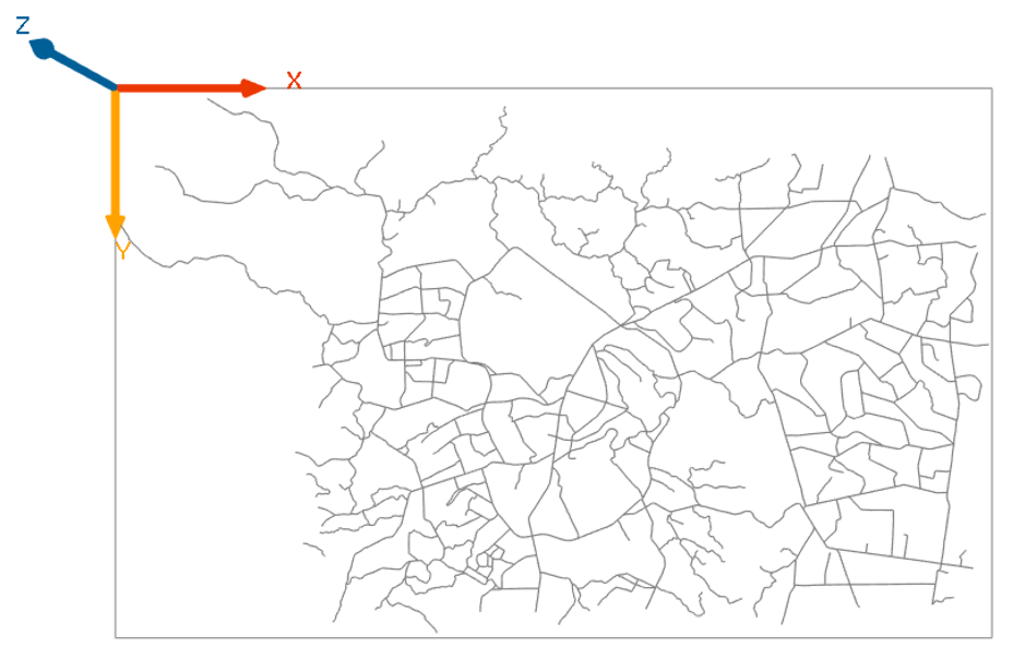
If we run the plota_a_rodovia experiment (a green button should automatically appear with this name if there is no compilation error), we will see that nothing happens. This is because we did not say who should be created nor how many agents should be created. In our case, we must create all the desired highways, which will be an agent type. So we need to use the create command within init.
Init represents a set of actions that occur only once when the simulation is created. Init, because it is not a specific command of any agent, but of the universe, is inside global.
global{
	file shape_file_roads <- ("../includes/rodoviasdf.shp");
	geometry shape <- envelope(shape_file_roads);
	init {
		create rodovia from: shape_file_roads;
		}
	}
Clearing data for the streets
Streets cannot just be plotted on our map so that they can be navigable streets. We therefore need to turn the streets into graphs with their connections working like us. To do this, we need to take a few steps to ensure that we have a graph that connects all points, avoiding impossible scripting errors (no path between two points), loose streets (not at all connected to the graph) or simply file defects (streets 2 meters away from reality, creating a non-existent spacing).
Thus, before creating the streets of the imported file, we need to use a function specifically designed to clear this data before creating the highway agent: clean_network (street, tolerance, joins overlaps, maintains a single graph).
global{
	file shape_file_roads <- ("../includes/rodoviasdf.shp");
	geometry shape <- envelope(shape_file_roads);
	init {
		list<geometry> var0 <- clean_network(shape_file_roads.contents, 10, true, true);
		create rodovia from: var0;
		}
	}
So we created a list of temporary geometries, which we use to then create the streets.
However, we are leaving some information out when we do not analyze the number of lanes and lanes. To do this, we can simply use the information that is already in the GIS files and create a variable for each street with this attribute using the command: with: [variable :: format (search (column_name)), …].
global{
	file shape_file_roads <- ("../includes/rodoviasdf.shp");
	geometry shape <- envelope(shape_file_roads);
	init {
		list<geometry> var0 <- clean_network(shape_file_roads.contents, 10, true, true);
		create rodovia from: var0 with: [lanes::int(read("nrfaixas")),vias::int((read("nrpistas"))];
		}
	}

species rodovia {
		int vias;
		int lanes;
		aspect base {
			draw shape color: #gray;
			}
		}
Next we need to ensure that there is a pathway for each direction of the track, as the tracks must be directional. Thus, for each track, there must be another one of equal properties and inverted geometry. In addition we need to explicitly ensure that the streets are connected to each other. When we call an agent within the role of another agent, we refer to the newer as self, and the oldest to myself (who called the function first).
global{
	file shape_file_roads <- ("../includes/rodoviasdf.shp");
	geometry shape <- envelope(shape_file_roads);
	init {
		list<geometry> var0 <- clean_network(shape_file_roads.contents, 10, true, true);
		create rodovia from: var0 with: [lanes::int(read("nrfaixas")),vias::int((read("nrpistas"))]{
			create rodovia {
				lanes <- myself.lanes;
				shape <- polyline(reverse(myself.shape.points));
				linked_road <-myself;
				myself.linked_road <- self;
		}}}}

species rodovia skills: [skill_road]{
		int vias;
		int lanes;
		aspect base {
			draw shape color: #gray;
			}
		}
Now that we have the links from our graph, we just need the nodes. To create the node, we create a temporary line graph, then pass each vertex and create a node agent at that location.
global{
	file shape_file_roads <- ("../includes/rodoviasdf.shp");
	geometry shape <- envelope(shape_file_roads);
	init {
		list<geometry> var0 <- clean_network(shape_file_roads.contents, 10, true, true);
		create rodovia from: var0 with: [lanes::int(read("nrfaixas")),vias::int((read("nrpistas"))]{
			create rodovia {
				lanes <- myself.lanes;
				shape <- polyline(reverse(myself.shape.points));
				linked_road <-myself;
				myself.linked_road <- self;
		}}
		graph tenp_graph <- as_edge_graph(rodovia);
		loop v over: temp_graph.vertices {
			create no with: [location::point(v)];
			}
		}}

species no skills: [skill_road_node];
.
.
.
To merge the links and nodes into a steerable graph, we declare a global graph (since it will be used outside init) and use the as_driving_graph() function to return the graph by joining lines and nodes.
global{
	file shape_file_roads <- ("../includes/rodoviasdf.shp");
	geometry shape <- envelope(shape_file_roads);
	init {
		list<geometry> var0 <- clean_network(shape_file_roads.contents, 10, true, true);
		create rodovia from: var0 with: [lanes::int(read("nrfaixas")),vias::int((read("nrpistas"))]{
			create rodovia {
				lanes <- myself.lanes;
				shape <- polyline(reverse(myself.shape.points));
				linked_road <-myself;
				myself.linked_road <- self;
		}}
		graph tenp_graph <- as_edge_graph(rodovia);
		loop v over: temp_graph.vertices {
			create no with: [location::point(v)];
			}
		the_graph <- as_driving_graph(rodovia, no);

		}}
.
.
.
To create the cars, we need to define some basic elements such as the amount of cars, location and top speed. Here, the initial location will be given by a random node, and the speed and number of cars will be fixed integers, for simplicity. To ensure that the car starts correctly in our system, we must create a random target and calculate its path with the compute_path() function.
create carro number:10{
	location <- one_of(no).location;
	max_speed <- 80.km/.h;
	no the_target <- one_of(no);
	try(do compute_path(graph: the_graph, target:the_target);
	}
Considering that we must also define the agent (client-person), we have to make it clear that we want to use the advanced_driving attribute by calling it. To define a function that will be called every tick, we use the term reflex. Here we will make the cars drive randomly on each tick.
species carro skills: [advanced_driving]{
	reflex andar_aleatorio {
		do drive random;
	}

	aspect base {
		draw sphere(50) color: #yellow;
	}
}
The visual result of this model is this:
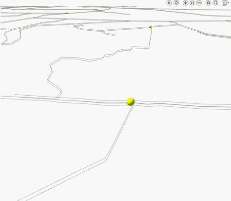
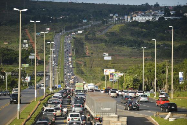
Analyzing the equivalent of the colorado descent (A quite busy road in Brasília), we noticed a higher vehicle density in this area.
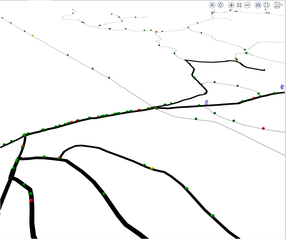
In fact, the region is one of the busiest in the city, and is even undergoing a work of expansion expected to end in 2019.
Simulations like this could be used for a variety of purposes. Following the example above, we could use this simulation to analyze traffic if we added one more road in another location, or if we wanted to observe the effect of widening existing roads.
Model extension
This was the basis of the model for traffic simulation in real world cases. It is noteworthy that, although modeling using the advanced driving skill package is relatively complex, the results are much more reliable due to the dozens of attributes that are inherited automatically, such as braking inertia, probability of breaking the car (as a result of an accident), distance from the vehicle ahead, top speed and many others. To check out the article on advanced driving skill, read Traffic simulation with the RANGE platform.
However, it is important to consider that models using simpler packages can have as positive results as the ones presented here. On the platform’s website, a quick tutorial teaches you how to set up a traffic analysis model in a city where residents have a home address, and a workplace. The model, by using a simpler skill package (moving skill) is able to generate this scenario with relative simplicity.