SVM Tutorial
In this tutorial we will present a general introduction of Support Vector Machines (SVM) and a basic application using the package e1071.
What is Support Vector Machine?
Support Vector Machine was developed in the study of Boser, Guyon e Vapnik in 1992. It is a supervised learning algorithm that aims to classify a certain set of data points that are mapped to a multidimensional feature space using a kernel function, the approach used to classify problems. In this case, the decision boundary in the input space is represented by a hyperplane in a larger dimension in space (VAPNIK et al., 1997 and SARADHI et al., 2005).
Simplifying…
SVM performs the separation of a set of objects with different classes, in other words, it uses the concept of decision plans.
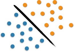
We can analyze the use of SVM with the following example. It is possible to observe in Figure 1 two classes of objects: blue or orange. This line that divide them defines the boundary between the blue dots and the orange dots. When entering new objects in the analysis, these will be classified as oranges if they are to the right and as blue if they are on the left. In this case, we were able to separate, through a line, the set of objects in their respective group, which characterizes a linear classifier.
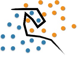
However, classification problems are usually more elaborate, and it is necessary to perform optimal separation through more complex structures. The SVM proposes to classify new objects (test) based on available data (training). This can be seen in Figure 2. The optimal separation in this case would occur with the use of a curve.
On the left of Figure 3 we observe the complexity in separating the original objects. To map them, we use a set of mathematical functions, acknowledged as Kernels. This mapping is known as the process of object reorganization.
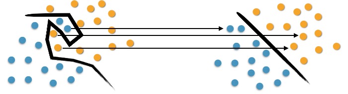
We can observe in the right of Figure 3 that there is a linear separation between objects. Thus, instead of constructing a complex curve, as in the left scheme; the SVM proposes, in this case, an optimum line capable of separating the blue points from the oranges.
And now, how can I apply this model?
First, it is necessary to load the data that will be studied. Luckily, this dataset is already natively available in R. To load it, simply run the following command:
data(iris)
After loading the database we will do some explorations:
summary(iris)
head(iris)
tail(iris)
str(iris)
The summary() command presents some statistics of the dataframe variables, such as mean, median, maximum, minimum and quantiles.
>summary(iris)
  Sepal.Length    Sepal.Width     Petal.Length    Petal.Width          Species
 Min.   :4.300   Min.   :2.000   Min.   :1.000   Min.   :0.100   setosa    :50
 1st Qu.:5.100   1st Qu.:2.800   1st Qu.:1.600   1st Qu.:0.300   versicolor:50
 Median :5.800   Median :3.000   Median :4.350   Median :1.300   virginica :50
 Mean   :5.843   Mean   :3.057   Mean   :3.758   Mean   :1.199
 3rd Qu.:6.400   3rd Qu.:3.300   3rd Qu.:5.100   3rd Qu.:1.800
 Max.   :7.900   Max.   :4.400   Max.   :6.900   Max.   :2.500
The head() and tail() commands show the first and the last six lines in this order. The str() command displays the structure of the variables. For example, if they are quantitative or categorical.
> head(iris)
  Sepal.Length Sepal.Width Petal.Length Petal.Width Species
1          5.1         3.5          1.4         0.2  setosa
2          4.9         3.0          1.4         0.2  setosa
3          4.7         3.2          1.3         0.2  setosa
4          4.6         3.1          1.5         0.2  setosa
5          5.0         3.6          1.4         0.2  setosa
6          5.4         3.9          1.7         0.4  setosa
From this, it is possible to have a sense about the data structure and which types of variables we will work with. It is very important to know the data that will be used.
Since we will use the quantitative variables ‘Sepal Length’, ‘Sepal Width’, ‘Petal Length’ and ‘Petal Width’ as predictors for the categorical variable ‘Species’, it is interesting to observe the correlation between the model covariables.
> names(iris)
[1] "Sepal.Length" "Sepal.Width"  "Petal.Length" "Petal.Width"  "Species"

> cor(iris[,1:4])
             Sepal.Length Sepal.Width Petal.Length Petal.Width
Sepal.Length    1.0000000  -0.1175698    0.8717538   0.8179411
Sepal.Width    -0.1175698   1.0000000   -0.4284401  -0.3661259
Petal.Length    0.8717538  -0.4284401    1.0000000   0.9628654
Petal.Width     0.8179411  -0.3661259    0.9628654   1.0000000
The charts tell stories!
Charts are an excellent tool to abstract and present your explorations. Studies that reach most spectators are those which use all possible resources to make the information as intelligible as possible. Let’s visualize how each variable is related by a gradient map, defining red (warm color) for greater correlation between the variables and blue (cold color) for lower correlation:
library(lattice)
cor <- cor(iris[,1:4])
rgb.palette <- colorRampPalette(c("blue", "red"), space = "rgb")
levelplot(cor, main="Correlation Iris Dataset", xlab="", ylab="", col.regions=rgb.palette(120))
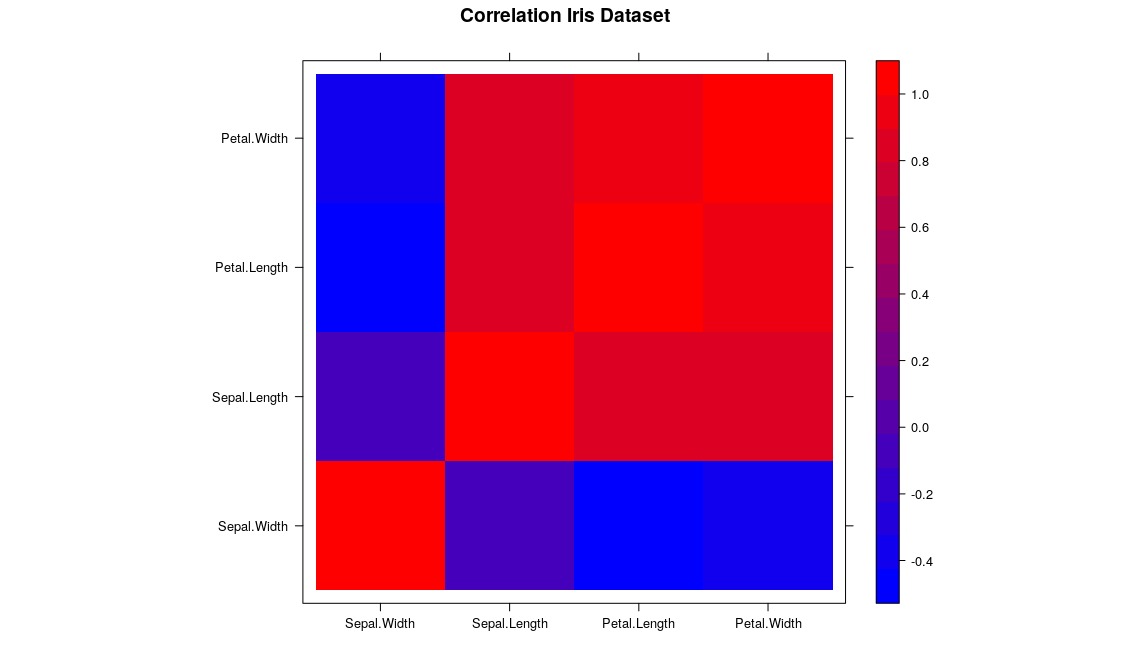
A nice correlation chart ![]() . First we import the
. First we import the lattice library which is responsible for generating our graph, store a correlation matrix in a variable and then create a color scheme (an array with a computational definition of these colors) with a ColorRampPaletter() function, going From blue to red. Finally we give these definitions to the function levelplot() that will take care of the rest.
Now we will present the definitive chart to understand our data, the three-dimensional scatter chart. We have four variables but only 3 will allow us to see beyond!
install.packages("scatterplot3d")
library(scatterplot3d)
colors <- c("#e41a1c", "#377eb8", "#4daf4a")
colors <- colors[as.numeric(iris$Species)]
scatterplot3d(iris[,1:3], pch = 15, color=colors)
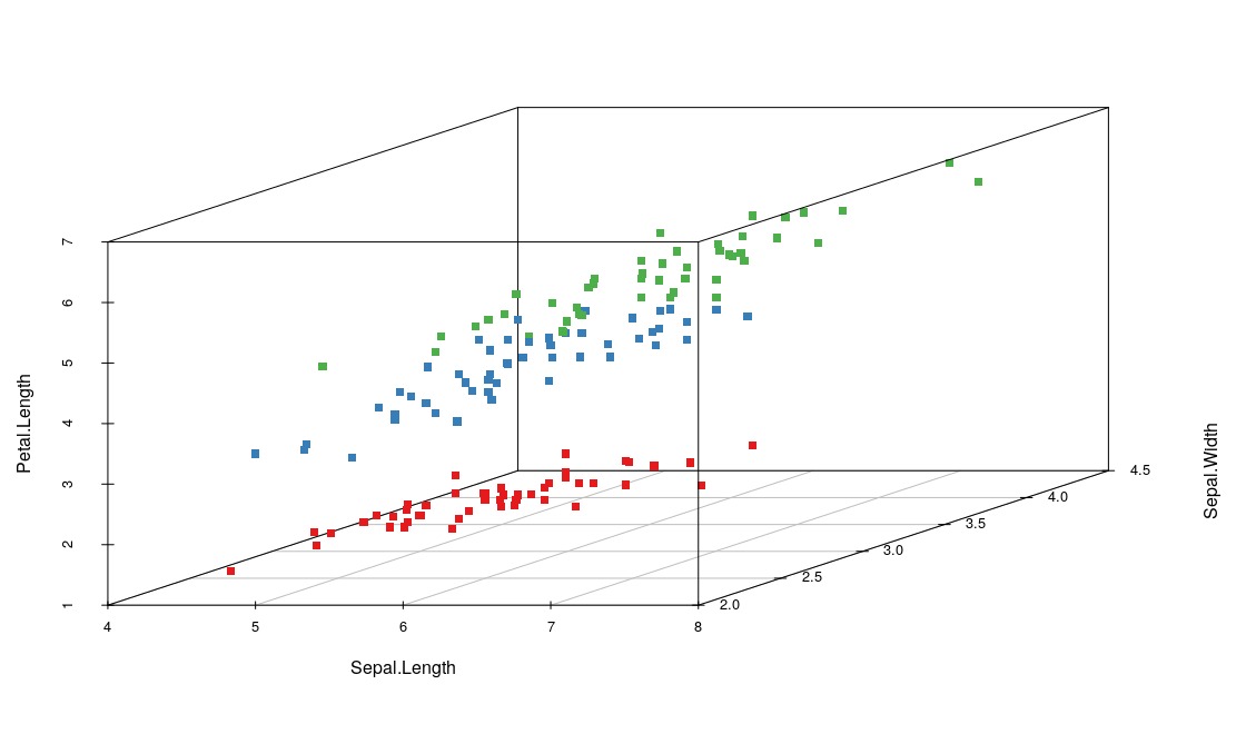
After installing and loading the scatterplot3d, we define 3 hexadecimal colors and save in the colors array, so we overwritten this array with an array referring to the species and replacing it by the color. Species 1, color 1, species 2, color 2… Finally, we pass all these parameters to our function that generates our graph. As you can see, a ‘separation’ is clear for our data, so it will not be a difficult job for our machine.
Now the most expected part… #letsgo
To use SVM, you need to install the e1071 package using the install.packages("e1071") command.
Wait to finish the installation process and let’s separate the data.
First, we will separate 70% of the observations from our dataset to ‘calibrate’ the model and use the other observations to verify the predictive power of the adjusted model.
> dim(iris)
[1] 150   5

> treino <- sample(1:150, 0.7*150)
> teste <- setdiff(1:150,treino)

> iris_treino <- iris[treino,]
> iris_teste <- iris[teste,]
In the e1071 package, we use thesvm() function to adjust the support vector machine model. Note that the syntax is quite similar to the lm() and glm() functions for linear and generalized linear models. Once we declare the dependent variable (the variable in which we want to make predictions), the function will automatically detect its type (categorical or quantitative) and use the appropriate procedure to fit the model.
> require(e1071)
> modelo1 <- svm(Species ~ . , data = iris_treino)

> summary(modelo1)
Call:
svm(formula = Species ~ ., data = iris_treino)


Parameters:
   SVM-Type:  C-classification
 SVM-Kernel:  radial
       cost:  1
      gamma:  0.25

Number of Support Vectors:  49
We used the “radial” kernel in the proposed model, since it is the default (which the function admits if nothing in the argument is informed). The svm() function accepts the following kernels: radial, linear, polynomial, and sigmoid.
Different kernels fit different models and, consequently, different predicted values. We will then adjust one model for each kernel, aiming to obtain a lower rate of classification error.
modelo2 <- svm(Species ~ . , kernel = "linear" , data = iris_treino)
modelo3 <- svm(Species ~ . , kernel = "polynomial" , data = iris_treino)
modelo4 <- svm(Species ~ . , kernel = "sigmoid" , data = iris_treino)
We now apply the adjusted models in the observations of the ‘test’ base and, through a contingency table, compare the classification proposed by the models with the actual observations classification.
preditos1 <- predict(modelo1,iris_teste)

> table(preditos1,iris_teste$Species)

preditos     setosa versicolor virginica
  setosa         11          0         0
  versicolor      0         20         0
  virginica       0          1        13
When performing the same procedure for other models, we can use the sum of the elements that don’t belong to the main diagonal as a measure of error, since they correspond to elements that were misclassified.
preditos2 <- predict(modelo2,iris_teste)
preditos3 <- predict(modelo3,iris_teste)
preditos4 <- predict(modelo4,iris_teste)

t1 <- table(preditos1,iris_teste$Species)
t2 <- table(preditos2,iris_teste$Species)
t3 <- table(preditos3,iris_teste$Species)
t4 <- table(preditos4,iris_teste$Species)
> sum(c(t1[lower.tri(t1)],t1[upper.tri(t1)]))
[1] 1
> sum(c(t2[lower.tri(t2)],t2[upper.tri(t2)]))
[1] 1
> sum(c(t3[lower.tri(t3)],t3[upper.tri(t3)]))
[1] 3
> sum(c(t4[lower.tri(t4)],t4[upper.tri(t4)]))
[1] 7
Thus, we saw that model 1 (kernel = radial) and model 2 (kernel = linear) presented more satisfactory results, since they missed only one classification in the test base.
Conclusion
The SVM has a wide range of applications in several areas, such as finance, biology, medicine, logistics, among others.
This is due to its application advantages such as: good generalization performance; mathematical treatability; geometric interpretation and the use for the exploitation of unlabeled data (YANG et al., 2002).
This tutorial is only a small demonstration of how this powerful tool can be used. We hope it has been useful to our readers!
References
BOSER, B. E.; GUYON, I. M.; VAPNIK, V. N. A Training Algorithm for Optimal Margin Classifiers. In: ANNUAL WORKSHOP ON COMPUTACIONAL LEARNING, 5, 1992, Pittsburgh. ACM Press. Pittsburgh: Haussler D, jul 1992. p.144-152 .
DRUCKER, H.; BURGES, C. J.; KAUFMAN, L.; SMOLA, A.; VAPNIK, V. Support vector regression machines. Advances in neural information processing systems, Morgan Kaufmann Publishers, p. 155–161, 1997.
SARADHI, V., KAMIK, H., MITRA, P. A Decomposition Method for Support Vector Clustering. In Proc. of the 2nd International Conference on Intelligent Sensing and Information Processing (ICISIP), p. 268-271, 2005.