Event Study

Hello everyone! This week LAMFO brings to you the methodology known as Event Study, we will start with a breaf introduction, referencial and then an exemple using R.

Nowadays isn’t hard to hear or read news about events that change contries or the world. We receive updates, new information and opinions about different topics and we reflect it on our behavior and adjust our plans, but about the market? Do you think that it reacts about those event?

To answer this question was created the Event Study.

Methodology

The author Campbell, Lo and Mackinley (1997) were the firsts to define and write about this methodoly. The basic idea is to observe if the value of a company suffers a variation when a event appears, in other words, if the expected “normal return” if affected by an “annomaly”. The development of Event Study has it fundamentals on the Theory of Efficient Markets of Fama (1970), which believes that the markets absorbes the public information and reflects it in stocks prices.

Here are four simple steps to start an Event Study!

Step 1: Define the Event

But what kind of event are we talking about?

We can study any kind of event, we only need to have enough data and the event must be known by the public. As exemples of events we havey:

Dividends distribution;
Fusion or aquisition of other company;
Reaquisition of stocks;
New laws or regulations;
Privatization or nationalization;
Political scandals.

One the event has been chosen, a time line will be defined with the windows for analysis.

Estimation Window: this window stabilish the normal return expected from the company, from $T_0$ to $T_1$. Here we will have a standart to compare the event, since this data hasn’t been “contaminated” by the news of the event.

Event Window: here is the time where the news about the event get in. The zero moment ($0$) will be the exact date that the event came public, after that we stabilish a safaty window to be get the information leak before, from $T_1$ to $0$, and to be sure that the market has absorbed all the information, from $2$ to $T_2$

An important detail, there is no fixed number to create the safety window. We can choose three months, fifthteen days or one year before the event, one way to identify the best safety window is testing different periods and analyse the statistic error.

Pos Event Window: moment after the event and market position.

Step 2: Companies

Once the dates are difined, now we need to select the companies that will be analysed and why. Usually, the first option is to get companies with stock exchange, since the returns are easy to get.

The second filter may be the sector or area that the companies are. For exemple, if we were studying the impact of new environmental law, would be interesting select companies from oil or mining industry.

Now we need to colect the return data from those companies. Is important that the data time format be the same, if the event will be marked by a day so the data of the returns must be daily returns.

Step 3: Stabilish Normal Returns and Abnormal

Following the time line, we first calculate the normal return of the stocks so then we can analyse the anormality.

A data base with the returns is enough to start the building the normal returns base. Remeber that the time format must be the same and they start at $T_0$ and be over at $T_2$.

To verify the existence of abnormal returns, or not, we will use the equation:

\[Ra_{i,t}=R_{i,t} - \mathbb E[R_i|X_t ]\]

Where $Ra_{i,t}$ is the abnormal return, since it is the difference between the actual return in t($R_{i,t}$) and the normal return ($$E[R_i

X_t ]$$).

Once we already had the base with companies return from $T_0$ to $T_2$, we must choose the best model to stablish the standart return:

Constant Mean Return Model
Adjusted Market Return
Market Model
Economic Model

Constant Mean Return Model

The expected normal return is defined by a simple mean of the real return in the estimation window ($T_0$ a $T_1$).

\[Ra_{i,t}=R_{i,t} - \overline R_i\]

One critic to this model is that the assumption that the returns will be constants with the pass of time. In some time formats, where the volatility is high, this characteristic alrady has a problem.

Adjusted Market Return

This case, the normal return will be difined by the return of the market portfolio ($Rm$). This method will require a new data base, in the same time format, from a benchmark.

\[Ra_{i,t}=R_{i,t} - Rm_i\]

Market Model

The Market Model has it base on statistic, representing an upgrade from the previous model.

Different from the Adjusted Market Return, the Market Model don’t set as default a market portfolio, but it uses an index such as S&P500 for north-america analysis or IBOVESPA for Brazilian stocks, been defined by:

\[Ra_{i,t}=R_{i,t} - \widehat \alpha_i - \widehat \beta_iR_{m,t}\]

The abnormal return ($Ra_{i,t}$) is defined by the difference from the real return of the asset in t and the parameters alpha ($\alpha$) and beta ($\beta$), estimated by a linear regression in the estimation window.

Using the linear regression in this model represent a big step in forecasting, since it depends on $R^2$. The bigger the $R^2$, less variance the abnormal return will have and more accurate the model will be.

Economic Models

Based on the market actions and since our objective is to etimate the stock future return, there are two methodologies available: (1) Capital Asset Pricing Model (CAPM) and (2)Arbitrage Princing Theory (APT). Both of them may be used to the calculus of normal returns, but with their requisits.

Capital Asset Princing Model (CAPM)

\[Ra_{i,t} = R_i - Rf_i - \beta (Rm_i - Rf_i)\]

The abnormal return is the result of the difference between the real return and the estipulated return, considering the sensibility of the asset and market retun ($Rm$) and free risk assets returns ($Rf$).

Arbitrage Pricing Theory (APT)

\[Ra_{i,t} = R_i - R_f + \beta_1 R_1 + \beta_2 R_2 + \beta_n R_n\]

In this model, we have different risk prizes for different factos, each one with a specific sensibility, this mean that each factor has a beta. To aquire the betas ($\beta_n$) will be needed to do a linear regression for factor and asset.

Step 4: Measuring and Analyse the Abnormal Returns

When the model is set, we are ready to calculate the returns. Usually, we analyse the mean of abnormal return and the accumulative abnormal return.

To validate the results, look the P-VALOR of the model and the $R^2$. Both of them must be statistic relevant.

Applying the model

This exercise will be done using R, the following packages are recommended:

quantmod : colect financial data from companies.
eventstudies : automatic package to this methodology
zoo : data base treatment.
xts: treatment of temporal data without ajusts.

Housing Bubble in USA (2008) effects on Brazilian Companies

We will use the package of Event Study already created in R and after compare the results with the manual estimation of event study. Once we are analysing an economic event in housing sector, we will look for companies with stocks listed in the market (BM&FBOVESPA) and are in the sector. Since this is a simple exercise, we got two companies: Gafisa and Cyrela, and as a parameter for the Market Model the index IBOVESPA.

Event Study using the package eventstudies

The package is divided in steps, the first one is stabilish the name and the date that the event occured. Since the event is the same for both of them, we will input “2008-03-13” that is the approximently the date that the event came public.

#Step 1: List the assets and the date of the event
eventsDates<-data.frame("name"=c("BVSP","GAFISA","CYRELA"),
                         "when"=c("2008-03-13","2008-03-13","2008-03-13"))

#Step 2: Convert the text
eventsDates$name<-as.character(eventsDates$name)
eventsDates$when<-as.character(eventsDates$when)

#Step 3: Return Lists
BVSP<- read.csv("^BVSP.csv")
BVSP<-BVSP[,c(1,6)]
colnames(BVSP)<-c("Date","BVSP")

GAFISA<- read.csv("GFSA3.SA.csv")
GAFISA<-GAFISA[,c(1,6)]
colnames(GAFISA)<-c("Date","GAFISA")

CYRELA<- read.csv("CYRE3.SA.csv")
CYRELA<-CYRELA[,c(1,6)]
colnames(CYRELA)<-c("Date","CYRELA")

#Step 4: Merge the data bases
data<-merge(BVSP,GAFISA,by="Date",all=T)
data<-merge(dados,CYRELA,by="Date",all=T)

#Step 5: Calculate the return
data$BVSP <- c(NA,diff(log(as.numeric(data$BVSP)), lag=1))
data$GAFISA <- c(NA,diff(log(as.numeric(data$GAFISA)), lag=1))
data$CYRELA <- c(NA,diff(log(as.numeric(data$CYRELA)), lag=1))

#Step 6: Convert into zoo objects
data.zoo<-read.zoo(data)

#Step 7: Event Study Market Model
es.mm <- eventstudy(firm.returns = data.zoo,    #Returns base
                     event.list = eventsDatas,  #Event Dates
                     event.window = 5,          #Safety Window size   
                     type = "marketModel",      #Abnormal return model
                     to.remap = TRUE,           #Recalculate the return using cumsum
                     remap = "cumsum",          #Accumulative return
                     inference = TRUE,          #Inference of the event
                     inference.strategy = "bootstrap",   #Boostrap to standert error
                     model.args = list(market.returns=dados$BVSP))  #Data base with the index IBOVESPA
#Step 8: Plot event study
plot(es.mm)

#Step 9: Results
summary(es.mm)

As results we have:

Event outcome has 3 successful outcomes out of 3 events: 
[1] "success" "success" "success"

Aparently the bubble in USA has effected the return in Brazilian companies, but the result is significant? Let’s look into the graphic:

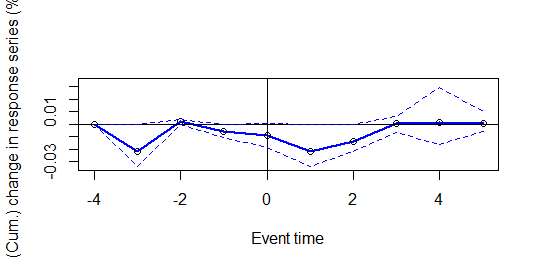
The blue line represent the companies’ return, and since is inside the abnormal area (doted lines) it shows the anormality of the series. However, the five days windw presents results equal zero, this mean that even if the event appears to cause disturbance in the series, it isn’t statistic significant.

Now, let’s calculate withou the package!

Event Study by hand

rm(list=ls())
library(quantmod)
GFSA<-read.csv("GFSA3.SA.csv")
CYRE<-read.csv("CYRE3.SA.csv")
BVSP<-read.csv("^BVSP.csv")

#Convert the date
GFSA$Date<-as.character(GFSA$Date)
GFSA$Date<-as.Date(GFSA$Date,format="%Y-%m-%d")
GFSA <- xts(GFSA[,-1], order.by=GFSA[,1])

CYRE$Date<-as.character(CYRE$Date)
CYRE$Date<-as.Date(CYRE$Date,format="%Y-%m-%d")
CYRE <- xts(CYRE[,-1], order.by=CYRE[,1])

BVSP$Date<-as.character(BVSP$Date)
BVSP$Date<-as.Date(BVSP$Date,format="%Y-%m-%d")
BVSP <- xts(BVSP[,-1], order.by=BVSP[,1])

#Bubble in 2008
startEvent = as.Date("2008-03-13") 

#Stabilish the window
endEvent = as.Date("2008-03-18") 

#Start of the series
startDate<-as.Date("2008-01-01")

#Calculate the log-retorn.
diffGFSA<-diff(log(GFSA$Adj.Close))
diffCYRE<-diff(log(CYRE$Adj.Close))

#Plot the adjusted close series
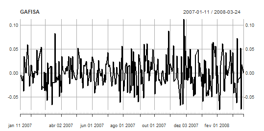
plot.xts(diffGFSA,major.format="%b/%d/%Y",
         main="GAFISA",ylab="Log-return Adj.Close price.",xlab="Time")

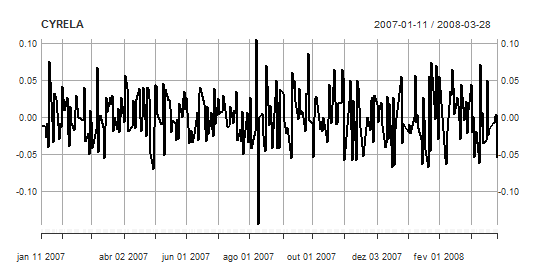
plot.xts(diffCYRE,major.format="%b/%d/%Y",
         main="CYRELA",ylab="Log-return Adj.Close price.",xlab="Time")

#Estimation Window
GFSASubset<-  window(diffGFSA, start = startDate, end = startEvent-1)
CYRESubset<-  window(diffCYRE, start = startDate, end = startEvent-1)

#BVSP
diffBVSP<-diff(log(BVSP$Adj.Close))
BVSPSubset<-window(diffBVSP, start = startDate, end = startEvent-1)

#Market Model
MarketModel<-lm(GFSASubset$Adj.Close~BVSPSubset$Adj.Close)
summary(MarketModel)

MarketModel2<-lm(CYRESubset$Adj.Close~BVSPSubset$Adj.Close)
summary(MarketModel2)

#Using Market Model
epsilon<-diffGFSA-coef(MarketModel)[1]-coef(MarketModel)[2]*diffBVSP

epsilon2<-diffCYRE-coef(MarketModel2)[1]-coef(MarketModel2)[2]*diffBVSP

#Find epsilon's variance
BVSPSubset1<-na.omit(window(diffBVSP, start = startDate+1,
                           end = startEvent-1))

X<-as.matrix(cbind(rep(1,length(BVSPSubset1$Adj.Close)),BVSPSubset1$Adj.Close))

BVSPSubset2<-window(diffBVSP, start = startEvent, end = endEvent)

Xstar<-as.matrix(cbind(rep(1,length(BVSPSubset2$Adj.Close)),BVSPSubset2$Adj.Close))

#GAFISA calculus
V<-(diag(nrow(X))*var(residuals(MarketModel)))+
  ((X%*%solve(t(Xstar)%*%Xstar)%*%t(X))*var(residuals(MarketModel)))

epsilonStar<-window(epsilon, start = startEvent, end = endEvent)
CAR<-sum(epsilonStar$Adj.Close)
SCAR<-CAR/sqrt(sum(V))

#CYRELA calculus
V2<-(diag(nrow(X))*var(residuals(MarketModel2)))+
  ((X%*%solve(t(Xstar)%*%Xstar)%*%t(X))*var(residuals(MarketModel2)))

epsilonStar2<-window(epsilon2, start = startEvent, end = endEvent)
CAR2<-sum(epsilonStar2$Adj.Close)
SCAR2<-CAR2/sqrt(sum(V2))

#Critical value of T distribution
alpha<-0.05
df<-length(GFSASubset$Adj.Close)-2
qt(alpha/2,df)
qt(1-(alpha/2),df)

df2<-length(CYRESubset$Adj.Close)-2
qt(alpha/2,df)
qt(1-(alpha/2),df)

The results for both companies are -2.012896 e 2.012896. Since wasn’t found any evidence in favor to reject the null hypothesis, the event has no significant impact over the compnies.

Finished this quick exercise about event study, in case of any doubt or for more info contact the LAMFO team!