Introduction
In this post, I intruduce the calculation measures of default banking. In particular, this post considers the Merton (1974) probability of default method, also known as the Merton model, the default model KMV from Moody’s, and the Z-score model of Lown et al. (2000) and of Tabak et al. (2013) , which is an adaptation of the Altman (1968) model.
The data used in the study are utilized in three stages. In the foreground, we use the values extracted from the balance of payments, then we use the financial statements, and lastly, we use the stock price history of world banks listed on the stock exchange, all extracted from the database of Bloomberg. The analysis period covers the first quarter of 2000 until the third quarter of 2016 with a periodicity of 67 quarters in 2,325 banks and 92 countries. Note that the assembled panel is unbalanced, containing 155,775 observations.
Merton Model
The Merton (1974) model aims to find the values of assets and their volatilities in a dynamic process following Black and Scholes (1973) . In the Merton model, it is assumed that the total value of the firm follows a geometric Brownian motion process.
\[dV = \mu Vdt +\sigma_V VdW\]where \(V\) is the total value of the firm’s assets (random variable), \(\mu\) is the expected continuous return of \(V\), \(\sigma_V\) is the firm value volatility, and \(dW\) is the standard process of Gauss–Wiener.
The Merton model uses the Black and Scholes (1973) model of options in which the firm’s equity value follows the stipulated process of Black and Scholes (1973) for call options. A call option on the underlying assets has the same properties as a caller has, namely, a demand on the assets after reaching the strike price of the option. In this case, the exercise price of the option equals the book value of the firm’s obligations. If the value of the assets is insufficient to cover the firm’s obligations, then shareholders with a call option do not exercise their option and leave the firm to their creditors.
\[E = V\mathcal{N}(d_1)- e^{-rT}F\mathcal{N}(d_2)\]where \(E\) is the market value of the equity of the firm (or free cash flow to the shareholder), \(F\) is the face value of the debt securities, \(r\) is the risk-free interest rate, and \(\mathcal {N} (.)\) is the standardized cumulative normal distribution; \(d_1\) is given by
\[d_1 = \frac{ln(\frac{V}{F})+(r+0.5\sigma^2_V)T}{\sigma_V\sqrt{T}}\]and \(d_2\) is simply \(d_1-\sigma_V\sqrt{T}\).
Applying the Itô Lemma in the dynamic process of \(V\) and manipulating the terms of Equation of \(d_1\), we obtain the following equation of the variability of the free cash flows of the shareholders (\(\sigma_E\)) (Bharath and Shumway, 2008) .
\[\sigma_E=\left(\frac{V}{E}\right)\frac{\partial E}{\partial V}\sigma_V\]Given that Merton (1974) , it can be shown that \(\frac{\partial E}{\partial V} = \mathcal{N} (d_1)\); then, Equation of \(\sigma_E\) can be written as follows (Bharath and Shumway, 2008) :
\[\sigma_E = \left(\frac{V}{E}\right)\mathcal{N}(d_1)\sigma_V\\]Basically, the algorithm works with Equations of \(E\) and \(\sigma_E\) to find the value terms of the asset \(V\) and the volatility of the asset value \(\sigma_V\). In this study, I use the Newton method to solve Equations \(E\) and \(\sigma_E\), the same algorithm that was used by Anginer and Demirguc-Kunt (2014) .
Equations \(E\) and \(\sigma_E\) have numerical solutions only for the values of \(V\) and \(\sigma_ {V}\). Once the numerical solution is found, the distance of default is calculated as follows:
\[DD = \frac{ln\left(\frac{V}{F}\right) + (\mu - \frac{1}{2}\sigma^{2}_{V})T}{\sigma_{V} \sqrt{T}}\]According to Bharath and Shumway (2008), the distance to the default model of Merton (1974) accurately measures the probability of firms defaulting.
\[\pi_{Merton} = \mathcal{N}(-DD)\]The default probability measure of Merton (1974) is simply the probability function of the normal minus the distance to default, Equation of $DD$. According to Bharath and Shumway (2008), this probability of default (Equation of \(\pi_{Merton}\)) should be a sufficient statistic for the default prognostic.
The starting point of the algorithm follows an adaptation of Bharath and Shumway (2008) and Anginer and Demirguc-Kunt (2014), where the initial kicks of \(V\) assume \(V = market \ capitalization + total \ liabilities\) and \(\sigma_ {V}\) assume \(\sigma_{V} = \sigma_{asset \ price \ return} \times (market \ capitalization + total \ liabilities).\)
Application in R
#######################
### Script Merton Model
#######################

## packages require

library(adagio)
library(nleqslv)
library(reshape2)
library(dplyr)
library(plyr)
library(pbapply)
library(stringdist)
library(xlsx)

# read the bank data
bank_panel_2000<- read.csv2("new_bank_panel_v18.csv",
stringsAsFactors=FALSE, sep = ";")

# make the DD_base
DD_base<- bank_panel_2000[,which(colnames(bank_panel_2000)%in%c("acao", "indice", "tempo", "quarter", "year", "cap_mercado", "passivo_total","retorno_med", "retorno_med_d",  "sd", "sd_d", "retorno_tri", "t_bill", "t") == TRUE)]

DD_base[which(colnames(DD_base)%in%c("acao", "indice", "tempo", "quarter") == F)][]<- lapply(DD_base[which(colnames(DD_base)%in%c("acao", "indice", "tempo", "quarter") == F)], as.numeric)

DD_base<- DD_base[complete.cases(DD_base), ]
DD_base<- DD_base[which(DD_base$passivo_total != 0), ]
DD_base<- DD_base[which(DD_base$sd != 0),]

# create the t variable in one quarter

DD_base$t = 1

##########################
##### p_merton ###########
##########################

# make the inicial p_merton

base_merton<- DD_base[,which(colnames(DD_base)%in%c("acao", "tempo", "quarter", "year") == TRUE)]
base_merton$valor_ativo_bailout<- NA
base_merton$vol_impl_ativo_bailout<- NA
base_merton$DD_merton_bailout<- NA
base_merton$p_merton_bailout<- NA


pb <- txtProgressBar(min = 0, max = nrow(base_merton), style = 3)
index <- 1

#i<- 1

for (i in 1:nrow(DD_base))
{


  D1<- DD_base$passivo_total[i]
  t<- DD_base$t[i]
  R<- DD_base$t_bill[i]
  Sigmas<- DD_base$sd[i]
  SO1<- DD_base$cap_mercado[i]

  fnewton <- function(x){
    y <- numeric(2)
    d1 <- (log(x[1]/D1)+(R+0.5*(x[2]^2))*t)/(x[2]*sqrt(t))
    d2 <- d1-x[2]*sqrt(t)
    y[1] <- SO1 - (x[1]*pnorm(d1) - (exp(-R*t))*D1*pnorm(d2))
    y[2] <- Sigmas*SO1 - pnorm(d1)*x[2]*d1
    y
  }

  xstart <- c(DD_base$cap_mercado[i] + DD_base$passivo_total[i] , DD_base$sd[i]*((DD_base$cap_mercado[i] + DD_base$passivo_total[i])))
  var_temp_merton<- nleqslv(xstart, fnewton, control=list(btol=.01), method="Newton")
  base_merton$valor_ativo_bailout[i]<- var_temp_merton$fvec[1]
  base_merton$vol_impl_ativo_bailout[i]<- var_temp_merton$fvec[2]


  # DD
  DD<- (log(base_merton$valor_ativo_bailout[i]/D1)+(DD_base$retorno_tri[i]-(0.5*(base_merton$vol_impl_ativo_bailout[i]^2)))*t)/base_merton$vol_impl_ativo_bailout[i]*sqrt(t)
  base_merton$DD_merton_bailout[i]<- DD


  # p_merton
  p_merton_bailout<- pnorm(- base_merton$DD_merton_bailout[i])
  base_merton$p_merton_bailout[i]<- p_merton_bailout

  index <-index+ 1
  setTxtProgressBar(pb, index)
}
close(pb)

# clean the base_merton

base_merton[is.na(base_merton)] <- NA
base_merton$DD_merton_bailout[is.infinite(base_merton$DD_merton_bailout)]<- NA
KMV Model
The KMV model is calculated from the total value of the firm’s assets \(V\) and the volatility of the asset value \(\sigma_{V}\) from the iteration between Equations \(E\) and \(\sigma_E\). We can observe the same process in Merton (1974) Model.
\[DD_{KMV it} = \frac{(V_{it} - TL_{it})}{(V_{it} \cdot \sigma_{V it})}\]where \(V_ {it}\) represents the market value of asset \(i\) in period \(t\), \(\sigma_ {V it}\) represents the volatility of asset value \(i\) in period \(t\), and \(TL_ {it}\) is total liabilities to asset \(i\) in period \(t\). As indicated by Equation \(DD_{KMV it}\), with higher \(DD_ {kMV it}\), the distance to default from bank \(i\) in period \(t\) is greater.
To normalize the variable to have a parallel effect and correlation analysis, normalization similar that elaborated by Merton (1974) is used. In other words, the probability of default of the KMV model is
\[\pi_{kmv} = \mathcal{N}(-DD_{KMV})\]The default KMV measure is the normal probability function minus the default distance, as well as the Merton (1974) model.
Application in R
################################
######## kmv_model #############
################################

base_kmv = base_merton

base_kmv$kmv_model_bailout<- (base_merton$valor_ativo_bailout - DD_base$passivo_total)/(base_merton$valor_ativo_bailout*base_merton$vol_impl_ativo_bailout)

base_kmv$kmv_model_bailout[is.na(base_kmv$kmv_model_bailout)] <- NA

base_kmv$kmv_model_bailout[is.infinite(base_kmv$kmv_model_bailout)]<- NA

kmv_model<- base_kmv[,which(colnames(base_kmv)%in%c("acao", "tempo", "kmv_model_bailout") == TRUE)]

# kmv_normalized
kmv_model$p_kmv<- pnorm(- kmv_model$kmv_model_bailout)
Z-Score Model
Another way to measure the default is the Z-score indicator, similar to Lown et al. (2000) and Tabak et al. (2013). According to Lown et al. (2000) and Tabak et al. (2013), this indicator represents the probability of bank failure. The Z-score measure has the following formulation:
\[Z-score_{it}=\frac{ROA_{it}+EQUAS_{it}}{\sigma_{ROA_i}}\]where \(EQUAS = \left(\frac{E_{it}-E_{it-1}}{TA_{it}-TA_{it-1}}\right)\). In this model, \(E_ {it}\) represents bank equity \(i\) in period \(t\), \(E_{it-1}\) represents bank equity \(i\) in period \(t-1\), \(TA_ {it}\) represents total assets of bank \(i\) in period \(t\), and \(TA_{it-1}\) represents total assets of bank \(i\) in period \(t-1\).
Parameter \(ROA_ {it}\) is expressed as the following relation:
\[ROA_{it}=\frac{2\pi_{it}}{(TA_{it}-TA_{it-1})}\]\(ROA_ {it}\) is the return on assets in period \(t\) for bank \(i\) and \(\sigma_ {ROA it}\) is the standard deviation of \(ROA\) of bank \(i\) in period \(t\). As the formula indicates, the higher the Z-score value, the lower the probability of bank failure \(i\). For Tabak et al. (2013), the Z-score is a risk default measure accepted by the literature. The Z-score measures the number of standard deviations of \(ROA\) that must decrease in order for banks become insolvent, which can be interpreted as the inverse of the probability of insolvency (Tabak et al., 2013).
Both the default probability measure of Merton (1974) and the KMV measure have a direct relationship with the default, that is, the higher their values, the greater the likelihood of a financial institution falling. Meanwhile, the Z-score model has an inverse relationship with the default bank, that is, the higher its values, the more distant the bank is from the default. This inverse relationship between the Merton Models, Model KMV and Model Z-score occurs because the first two represent a normalization of the distances from the default, making them directly linked to the default. In the Z-score model, on the other hand, the relationship is inverse because it measures the distance from the default, that is, the probability of banks being further from the default and not the direct probability of default.
The Merton (1974) model and the KMV model are default proxies that do not directly calculate the probability of default, but rather measure it implicitly, by looking at bank liabilities and how the market prices these liabilities (Milne, 2014). According to Wang et al. (2017), to measure the default risk, a common proxy should not be used, but a flexible enough measure to quantify most firms in the market.
The Z-score model, despite being an accepted measure in the risk measurement literature, especially of bank risk, does not express the market relationship, but the banks’ accounting relationship.
Application in R
########################
### Script Z-Score Model
########################

# construct the temp ROA data

temp_bank_ROA<- bank_panel_2000[, c(1:3, 30)]

temp_bank_ROA$quarter<- substring(temp_bank_ROA$tempo, first = 1, last = 3)
temp_bank_ROA$year<- substring(temp_bank_ROA$tempo, first = 5, last = 8)

temp_bank_ROA<- arrange(temp_bank_ROA,acao, year, quarter)

temp_bank_ROA_duplic<- ddply(temp_bank_ROA, .(acao), transform, ativo_total = c( NA, ativo_total[-length(ativo_total)]))
temp_bank_ROA_duplic<-  temp_bank_ROA_duplic[, -c (4:6)]
temp_bank_ROA<- arrange(temp_bank_ROA,acao, year, quarter)

temp_bank_ROA<- merge(temp_bank_ROA, temp_bank_ROA_duplic, by.x=c("acao", "tempo"), by.y=c("acao", "tempo"), all.x=T,all.y=T)
rm(temp_bank_ROA_duplic)

# creat a for to make a ROA

acoes_list<- unique(temp_bank_ROA$acao)
tempo_list<- unique(temp_bank_ROA$tempo)

temp_ROA<- temp_bank_ROA[1,]
temp_ROA$at_ROA<- NA
temp_ROA<- temp_ROA[-c(1),]

pb <- txtProgressBar(min = 0, max = length(acoes_list), style = 3)
index <- 1

#i <- acoes_list[1]
#y<- tempo_list[1]
for (i in acoes_list)
{
  temp_assets<- temp_bank_ROA[which(temp_bank_ROA$acao == i),]
  temp_assets$at_ROA<- NA
    for(y in tempo_list)
    {

    if (y == "CQ1.2000")
    {
    temp_assets$at_ROA[which(temp_assets$tempo == y)]<- temp_assets$ativo_total.x[which(temp_assets$tempo == y)] * 2
    }else {temp_assets$at_ROA[which(temp_assets$tempo == y)]<- sum(temp_assets$ativo_total.x[which(temp_assets$tempo == y)], temp_assets$ativo_total.y[which(temp_assets$tempo == y)], na.rm = TRUE)}

    }
  temp_ROA<- rbind(temp_ROA, temp_assets)
  index <-index+ 1
  setTxtProgressBar(pb, index)
  }
close(pb)

temp_ROA<- temp_ROA[, -c(3:4, 7)]
temp_ROA$at_ROA[temp_ROA$at_ROA == 0]<- NA

# make a merge with the bank_2000

temp_bank_panel_2000<- merge(bank_panel_2000, temp_ROA, by.x=c("acao", "tempo"), by.y=c("acao", "tempo"), all.x=T,all.y=T)

temp_bank_panel_2000<- arrange(temp_bank_panel_2000,acao, year, quarter)

# make the ROA data - Lown (2007)

temp_bank_panel_2000$ROA<- (2*temp_bank_panel_2000$ni)/(temp_bank_panel_2000$at_ROA)

bank_panel_2000<- temp_bank_panel_2000

# remove the extra data

rm(temp_bank_ROA, temp_bank_ROA_duplic, temp_assets, temp_bank_panel_2000)


# construct the temp ROE data

temp_bank_ROE<- bank_panel_2000[, c(1:2, 10, 30:32)]

temp_bank_ROE_duplic<- ddply(temp_bank_ROE, .(acao), transform, patrimonio_liquido = c( NA, patrimonio_liquido[-length(patrimonio_liquido)]))
temp_bank_ROE_duplic<-  temp_bank_ROE_duplic[, c (1:3)]


temp_bank_ROE<- merge(temp_bank_ROE, temp_bank_ROE_duplic, by.x=c("acao", "tempo"), by.y=c("acao", "tempo"), all.x=T,all.y=T)

temp_bank_ROE<- arrange(temp_bank_ROE,acao, year, quarter)

rm(temp_bank_ROE_duplic)

# creat a for to make a ROE

acoes_list<- unique(temp_bank_ROA$acao)
tempo_list<- unique(temp_bank_ROA$tempo)

temp_ROE<- temp_bank_ROE[1,]
temp_ROE$at_ROE<- NA
temp_ROE<- temp_ROE[-c(1),]

pb <- txtProgressBar(min = 0, max = length(acoes_list), style = 3)
index <- 1

#i <- acoes_list[1]
#y<- tempo_list[1]
for (i in acoes_list)
{
  temp_assets<- temp_bank_ROE[which(temp_bank_ROE$acao == i),]
  temp_assets$at_ROE<- NA
  for(y in tempo_list)
  {

    if (y == "CQ1.2000")
    {
      temp_assets$at_ROE[which(temp_assets$tempo == y)]<- temp_assets$patrimonio_liquido.x[which(temp_assets$tempo == y)] * 2
    }else {temp_assets$at_ROE[which(temp_assets$tempo == y)]<- sum(temp_assets$patrimonio_liquido.x[which(temp_assets$tempo == y)], temp_assets$patrimonio_liquido.y[which(temp_assets$tempo == y)], na.rm = TRUE)}

  }
  temp_ROE<- rbind(temp_ROE, temp_assets)
  index <-index+ 1
  setTxtProgressBar(pb, index)
}
close(pb)

temp_ROE<- temp_ROE[, -c(3:7)]
temp_ROE$at_ROE[temp_ROE$at_ROE == 0]<- NA

# make a merge with the bank_2000

temp_bank_panel_2000<- merge(bank_panel_2000, temp_ROE, by.x=c("acao", "tempo"), by.y=c("acao", "tempo"), all.x=T,all.y=T)

temp_bank_panel_2000<- arrange(temp_bank_panel_2000,acao, year, quarter)

# make the ROE data - Lown (2007)

temp_bank_panel_2000$ROE<- (2*temp_bank_panel_2000$ni)/(temp_bank_panel_2000$at_ROE)

bank_panel_2000<- temp_bank_panel_2000

# remove the extra data

rm(temp_bank_ROE, temp_assets, temp_bank_panel_2000)

########################################################################################
########################### make the "Outdated" data ###################################
########################################################################################

bank_panel_2000$mtb<-((bank_panel_2000$ativo_total)/(bank_panel_2000$passivo_total))/(bank_panel_2000$cap_mercado)

# make a log(at)

bank_panel_2000$log_at<- log(bank_panel_2000$ativo_total)

# make a lev_ratio

bank_panel_2000$lev_ratio<- (bank_panel_2000$passivo_total/bank_panel_2000$patrimonio_liquido)

# make the EQAS variable

bank_panel_2000$EQAS<- bank_panel_2000$at_ROE/bank_panel_2000$at_ROA

# make the z-score variable

sd_roa<- ddply(bank_panel_2000, .(acao), summarize, sd_roa = sd(ROA, na.rm = TRUE))

sd_roa$sd_roa[is.na(sd_roa$sd_roa)] <- 0
sd_roa$sd_roa[sd_roa$sd_roa == 0]<- NA

temp_zscore_bank2000<- merge(bank_panel_2000, sd_roa, by.x=c("acao"), by.y=c("acao"), all.x=T,all.y=T)

bank_panel_2000<- temp_zscore_bank2000
rm(temp_zscore_bank2000)

bank_panel_2000$z_score<- (bank_panel_2000$ROA + bank_panel_2000$EQAS)/bank_panel_2000$sd_roa
A Cross-Country Application
In this section, I discuss the descriptive analyzes of the inputs that comprise the calculation of the default variables. In the foreground, I discuss the inputs that make up the default probability variable of Merton (1974) and the KMV model. The parameters are listed in Table 1. The inputs, as previously mentioned, follow the proposal of Bharath and Shumway (2008) and Anginer and Demirguc-Kunt (2014).
Tabel 1- Summary of Inputs in the \(\pi_{Merton}\) and KMV Models. All returns are continuos and monetary data are in milons of USD.
In the background, I approach the inputs that make up the variable Z-score of Lown et al. (2000) and of Tabak et al. (2013). The parameters are listed in Table 2.
Tabel 2- Summary of Inputs to \(Z-score\). All returns are continuos and monetary data are in milons of USD.
In Table 3 The values of the Merton (1974) model and KMV vary between \([0.1]\) probabilities of default. The values of the \(\log(Z-score)\) model are presented in values of deviations from default.
Tabel 3- Descriptive Analysis of Default Variables.
In Table 3 The values of the Merton (1974) model and KMV vary between \([0.1]\) probabilities of default. The values of the \(log(Z-score)\) model are presented in values of deviations from default.
As an illustration, Figure 1 shows the temporal evolution of the default indicators. It can be noticed that, near the period of the financial crisis of 2008, the indicators present a higher probability of default. The greater the \(\pi_ {Merton}\) indicator, the greater the probability that the bank defaults. The \(Z-score\) indicator is the inverse: the larger the indicator, the lower the probability of default. However, it is observed from Figure 1 that at some time points, the indicators move in the same direction. The \(Z-score\) indicator may have a slower response than the \(\pi_{Merton}\) indicator, since it has only accounting data sets, whereas the \(\pi_{Merton}\) indicator uses market data as well; these kind of data have faster responses to the default measures.
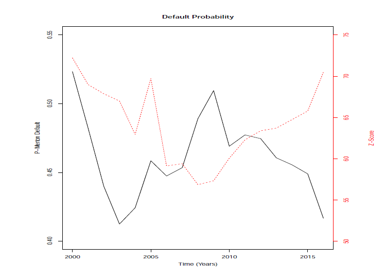 Figure 1: Temporal Evolution of the Default Measures
Another analysis was undertaken of the probabilities of default by economic region. Figure 2 shows the evolution of the average default probability of Merton (1974) in economic regions. It can be observed that in general, banks of North America, South Asia and Sub-Saharan Africa have higher indexes of default relative to other regions, such as Latin America, the Caribbean, North Africa, Middle East, Europe and Central Asia. This effect can be observed since, in general, regions that have the highest average indicators of default have larger numbers of financial institutions than do those of other regions.
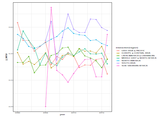 Figure 2: Temporal Evolution of Default Measures per Region
Final Remarks
In this post I show the main models of estimation and calculation of probability of default of banks. These measures are widely used in the scientific literature and practiced by financial institutions for making credit risk.
Such models usually work with the measurement of bank default taking credit risk into account, although banks are the main operating income there are other methods for banks to generate revenue, so these measures underreport the effects of these other forms of bank earnings.